![]()
![]()

Does Location Matter? – The Social Determinants of Spread of COVID-19
Introduction
While the very first case of infection by coronavirus will probably never really be accurately known, by the 31st of December 2019 the city Municipal Health Commission of Wuhan, a city in central China which lay at the junction of dense industrial and trade networks, reported an outbreak of cases of pneumonia. A new kind of coronavirus was subsequently identified. By mid-January, the first recorded cases were confirmed outside of China, starting with Thailand. On January 22, the WHO mission to China issued a statement stating that there was some evidence of human to human transmission, but more investigations were needed.
In the United States, the first confirmed case occurred on January 22, in King county, Washington, followed by Cook county in Illinois. The first confirmed death, as we know it today, occurred on 6 February in Santa Clara, California. As of June 1, there had been 103,717 deaths and 1,800,497 confirmed cases all over the US. The regional variation, the extent and intensity of both the spread of COVID cases and COVID related mortality, and the differences by state and county have been apparent right from the beginning. Since the origins of the virus lay outside the borders of the United States, the initial outbreaks were dependent on the “initial conditions”, and were locationally somewhat idiosyncratic. But over time, certain patterns have emerged, which we can analyze to detect location-specific attributes that have either aided or hindered the spread and impact of the virus.
As of June 1, only 197 of the 3195 US counties have been spared the scourge of the virus, and more than half – 1770 counties – have experienced at least one death from COVID. Figure 1 shows the top 5 counties with the highest prevalence rate among all counties in the nation in terms of confirmed cases per million, while Figure 2 shows the same for the top 10 countries with sizeable populations (over 100,000 people).
Figure 1
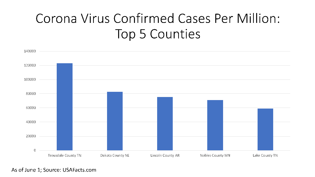
Figure 2
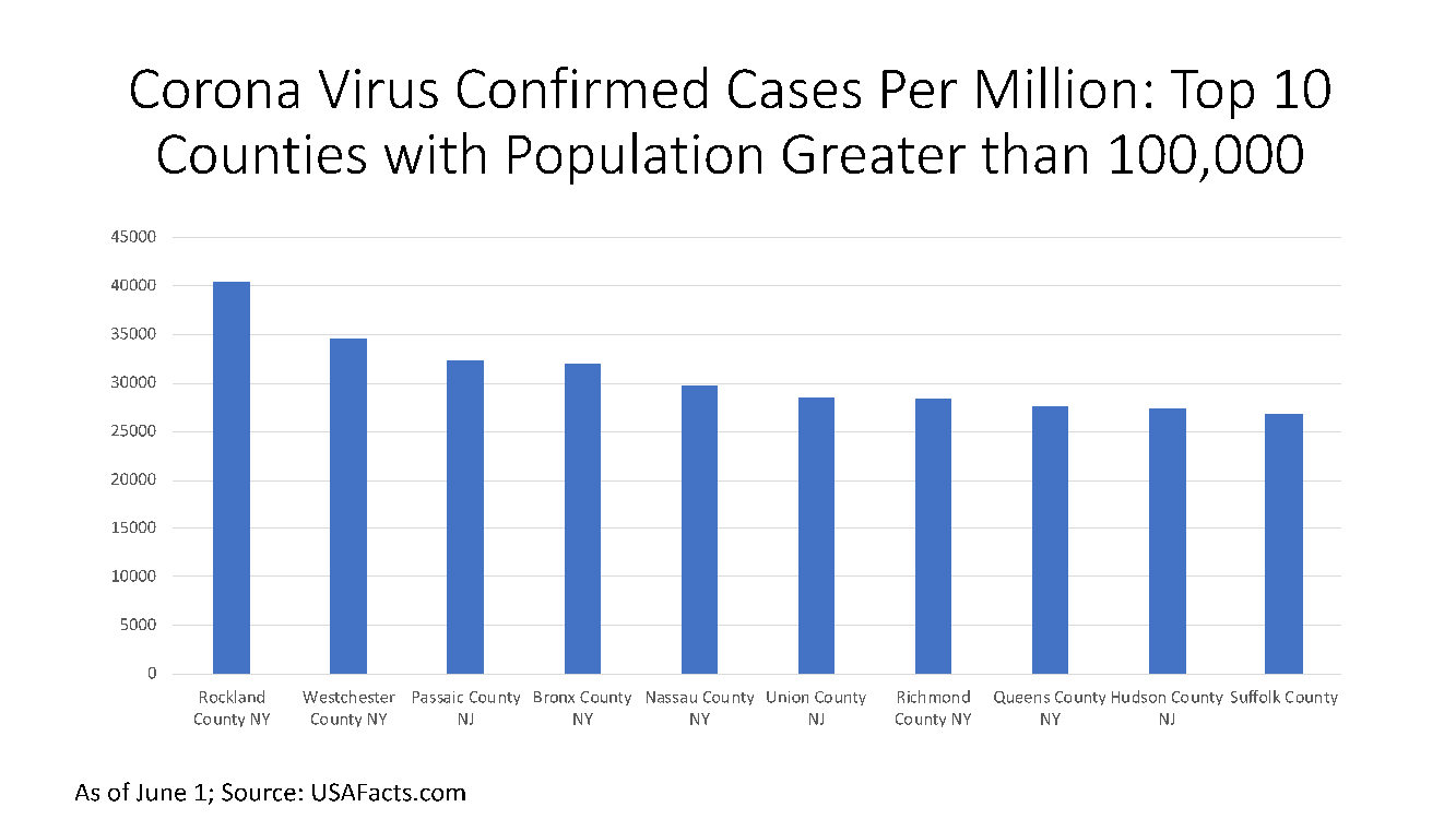
Figure 3

Motivation: The Social Factors Impacting Spread and Mortality
Figure 3 shows the top ten counties with the highest COVID mortality rates among counties with sizeable populations. Both flu/influenza and COVID have similar transmission channels when it comes to transference from person to person, with coughing, sneezing, and airborne infected droplets being the primary vehicles. Because the transmission for both is interpersonal, it is therefore socially “determined” and has significant externalities. For the sake of comparison, we show in Figure 3 the flu mortality rate superimposed on the top ten counties with highest COVID mortality rate. The transmission channels may be similar, but the geographic distribution of flu mortality is quite different. The highest flu mortality rates are in counties in Louisiana, South Carolina and Tennessee and the lowest in Collier County and Martin counties in Florida.
All the transmission factors mentioned above – coughing, sneezing, exposure to infected persons, etc. – suggest that there are network externalities that matter. Social interaction and networks are a mixed blessing: on one hand, they contribute to the spread; on the other, social relationships and community connections help provide mutual aid and support, which is vital at any time of crisis. There are attributes of the daily structures of social life, and the nature of built-up space, that predispose one to exposure and facilitate the spread of the virus. At the same time, there is increasing recognition that social connections among individuals – “social networks and the norms of reciprocity and trustworthiness that arise from them” have a salutary effect on many kinds of outcomes, including health related. Some specific features of localities and neighborhoods around the home – the socio-cultural ethos, economic and communal health and civic engagement – have a positive impact on health and in battling disease spread. In short, we attempt to tackle the question: what are the social determinants of the spread of COVID and what role do external, social factors play in determining both prevalence and mortality rate, over and above individual-specific physical, genetic, behavioral and other vulnerabilities?
Most of the debate hitherto, and understandably so, has revolved around the speed of the spread, the required preventive measures, the mode of transmission, the search for a vaccine, and projections of prevalence and mortality over time. Most of these and other epidemiological models are primarily time series models that forecast and predict spread based on parameters such as symptomatic or asymptomatic transfers, and reproduction numbers. However, the “cross-sectional” aspect, i.e. variation not over time, but over space, or the regional and local aspects of the spread of the virus has attracted attention only in so far as it focuses attention on the tragic situation in specific urban areas, such as New York.
Bubble develops health, life and homeowner risk analysis and scores for the insurance industry, taking into account both individual as well as external locality-based social and economic drivers affecting risks associated with home, and the life and health of individuals. We are not medical professionals, but the medical community has come to accept that where we live, and our social and environmental surroundings, impact our lifestyle, health-related behavior and hence, health outcomes. Bubble has therefore collected an extensive amount of local data impinging on these vital issues, for more than 3,000 counties and 30,000 zip codes across the US.
In this blog post, we take a cross-sectional view – snapshots at various points in time across the entire gamut of over 3,000 counties in the US, to analyze the local and county-level social determinants of the coronavirus spread. Does location matter for spread and for mortality, and if so, which social, environmental factors facilitate spread and which hinder it, and which community or socio-economic variables impact mortality positively or adversely? Since this is not an academic paper but rather a blog post, our objective here simply is to begin to demonstrate the salience of external factors and social interaction in the spread and impact of the virus.
Data
What are some of the influential local features and attributes that could impact the spread of the infection, given what we know about the transmission channels? A few obvious features have been mentioned in the media – e.g. the density of population and the frequency with which people collect in crowded spaces, whether for dining, sports or socio-cultural engagements. We proxy the duration and intensity of population interaction, through the reliance on public transportation and other metrics. On the other hand, we look at social cohesiveness, and proxy measures of mutual aid, support and assistance, such as inequality, segregation, and number of social associations. To provide a sense of the rich yield possible from the data, we highlight some sample statistics and charts that showcase key contextual features that are most relevant in the statistical models to follow:
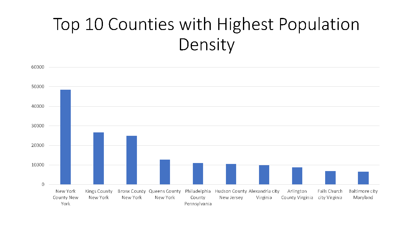
The most densely populated county in the US is New York county followed by Kings County and Bronx county with 48,600 people per square mile, 26,800 people per square mile and 25,000 people per square mile, respectively, while a number of counties in Alaska have the lowest densities (see Figure 4).
Figure 4
New York county also has the highest share (%) of people traveling by public transportation – which frequently throws people together in close proximity – with about 32% doing it regularly, followed by Kings County, NY with 28% and Queens county, NY with 25% (see Figure 5).
Figure 5
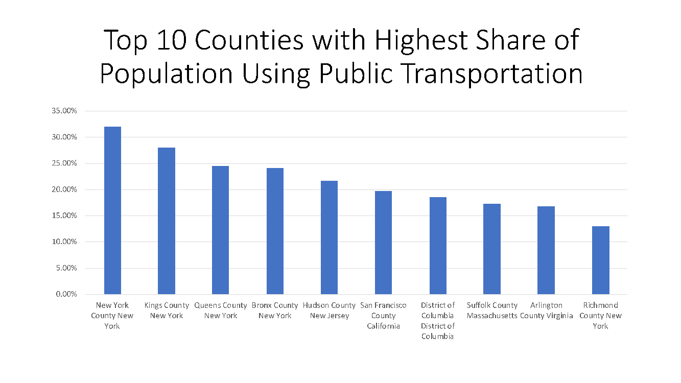
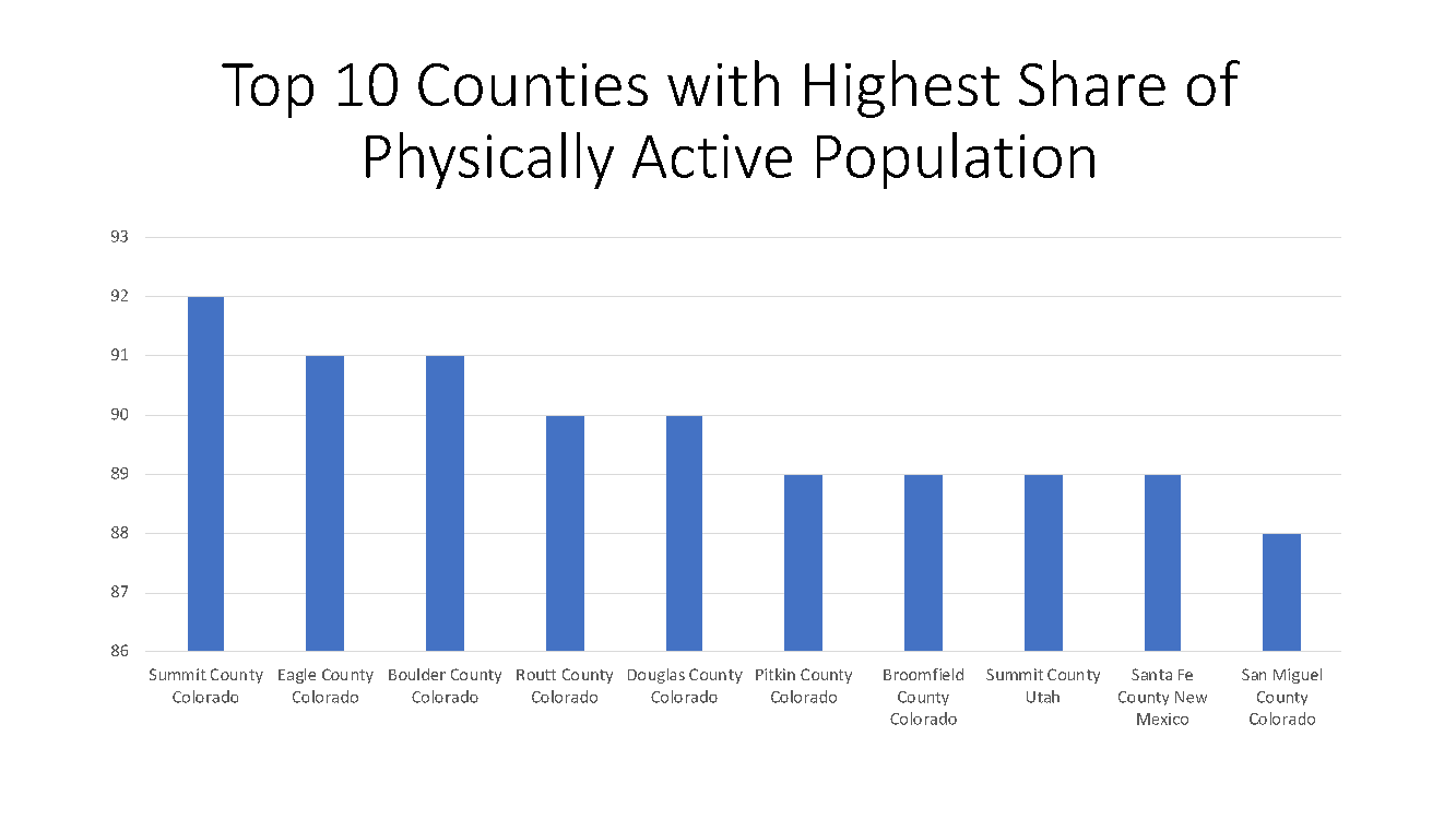
Figure 6 highlights the physically active nature of populations residing in the mountain states of Colorado, Utah and New Mexico. Physical activity is, of course, broadly recognized as a singularly effective lifestyle behavioral choice in promoting good health and fighting against any illness 1.
Figure 6
Income equality ratios and racial segregation indices are a measure of fractiousness of a community and hence its collective capacity to counter a local emergency. The former shows a wide geographic range with Eureka County in Nevada being the most unequal, followed by New York county and Clinch county, Georgia, while Roberts county, Texas and Wheeler county, Nebraska are those with very low-income inequality ratios. Figure 7 highlights the parts of the country with the highest measures of black-white residential segregation, which shows a very “diverse” range of counties in many different regions and states of the country.
Figure 7

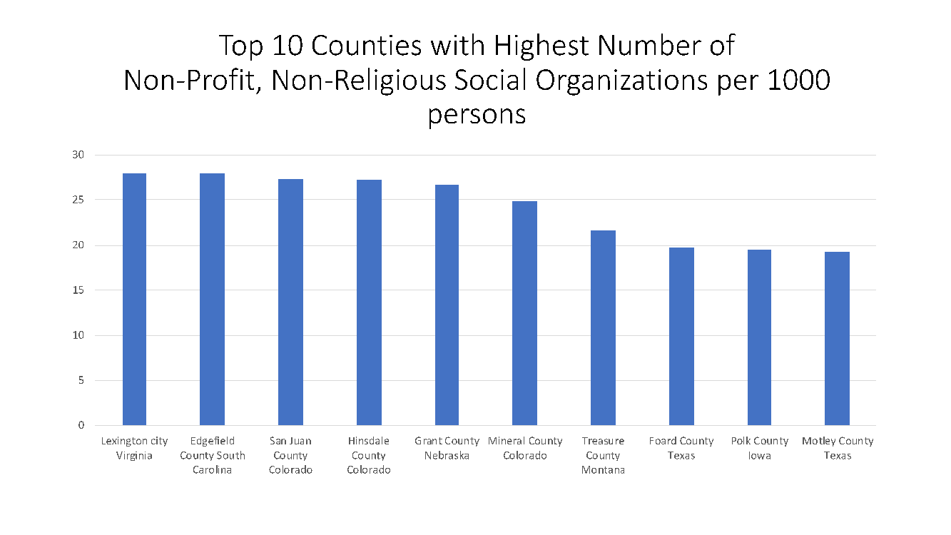
Figure 8 shows the counties with the highest number of social associations, societies, clubs and other such organizations, per 1,000 persons. Social associations are a measure of civic and civil society participation, important both as a metric of interaction (and hence, spread of infections), and for the probability of mutual aid and support which is relevant in lowering the mortality rate.
Figure 8
Many experts believe that places with higher concentrations of single-person households or smaller households stand a greater chance than places with larger households in stemming the spread of this infectious disease, because there are fewer persons to infect in closed indoor spaces. Figure 9 shows the top counties with the highest share of these smaller households.
Figure 9

Another example of a data vignette of relevance, and potentially associated with both the spread of the virus and the mortality rate, is the general level of affluence. While places with higher incomes have denser international linkages and more global travel, leading to higher probability of exposure, they also have resources to deal with the aftermath and during the treatment stage; a similar story can actually hold for dense urban networks. The Virginia counties on the outskirts of Washington DC, together with Santa Clara and San Mateo counties in Silicon Valley in California are among the most affluent in the country. As an apex measure of health, lifestyle and healthcare, life expectancy is the highest in San Miguel county, Colorado at 98 years and South Dakota has a cluster of three counties with the lowest life expectancy ranging between 62 and 65 years.
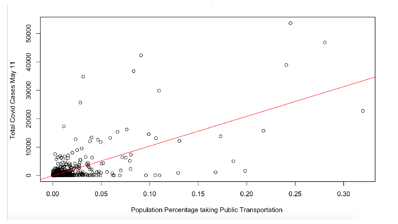
A quick look at the correlation of two of the causal factors listed above with the spread of the virus as of Monday, May 25 (we checked for every week starting in mid-April, and results are by and large the same) across the 3,000 plus counties, shows a positive relationship between population density and confirmed cases, as well as positive correlation between the share of the population taking public transportation and the number of confirmed cases (see Figures 10 and 11). Put simply, this suggests that higher confirmed cases are associated with counties that are densely populated and counties with higher usage of public transport, albeit without taking into account, as yet, any conflating factors. As the previous figures showed, urban counties in the New York metro area score high on both these counts, as well as on the prevalence of confirmed cases.
Figure 10. Confirmed COVID Cases vs Population Density
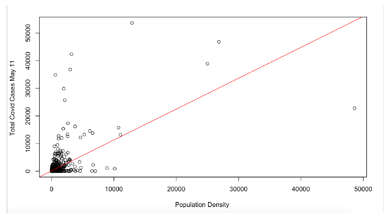
Figure 11. Confirmed COVID Cases vs Usage of Public Transportation
Discussion of COVID Prevalence and Mortality by County
We next run multivariate regressions on two different sets of dependent variables – a) on confirmed cases of Covid-19, and b) confirmed deaths from Covid-19. We recognize that confirmed cases is a crude variable and potentially biased by testing, for which we do not have reliable data for same granularity and frequency. Hence, the need to run mortality models that also include confirmed cases in recent past plus other variables. We ran the former for each Monday starting April 20 through May 11, and the latter starting three weeks later, from May 11 through June 1. An early sign that the results were robust and not a result of a momentary artifact of cross-sectional data was that we get similar results for each week for the dependent variable, with neither the signs of coefficients or the significance changing much. This seems to suggest a stable, time-invariant location specific social dynamic in the spread of the virus 2. The tables present the average coefficient magnitudes for the four weekly models. All the coefficients shown are significant at 95% confidence level.
For the first set of models on the determinants of Covid prevalence figures by county, some of our key independent variables of interest are those area-specific external social attributes that could have a bearing on the infection spread, such as population density, share of people taking public transportation, share of single-person households, and share of people with severe housing problems, while controlling for population, median household income, age distribution, share of people involved regularly in physical activity etc. Table 1 shows the averaged-out coefficients for the variables of interest. As expected, the independent variables that are positively associated with Covid cases are population density, the population share that takes public transportation and share of people in county with severe housing burden (a proxy for overcrowding, bad sanitation, poor kitchen facilities), while share of single person households is negatively associated with infection spread. The overall fit is quite good for a cross-sectional study and the results are robust 3. The coefficient magnitudes are not sizeable, except for the public transportation variable, which is particularly striking, with NY counties driving most of the result; excluding them still keeps the overall result but reduces the coefficient magnitude to the hundreds.
TABLE 1
Model for COVID Confirmed Cases
| Coefficient | |
| (Intercept) | -3350.74 |
| Percent with Severe Housing Burden | 27.53 |
| Percent Single Person Households | -27.40 |
| Proportion Using Public Transport | 66888.26 |
| Population Density per Sq.Mile | 0.14 |
| N=3123 | Adj R-squared: 0.61 |
Table 2 lays out the results of Covid confirmed death models averaged out over 4 weeks, as mentioned earlier. The first version of the model uses similar set of variables as for the models involving spread. Since mortality is a subset and nested within the larger infected population, we also use nested models, with the addition in the second specification, of confirmed cases three weeks before, as a predictor variable. Not surprisingly, the first model gives very similar results to the model of spread determinants in Table 1, with density, share of people regularly taking public transportation, percent of population as single person households and those with severe housing burden all behaving in a similar fashion.
TABLE 2
Model for COVID Deaths
| Estimate | |
| (Intercept) | -245.71 |
| Percent with Severe Housing Burden | 1.58 |
| Percent Single Person Households | -2.72 |
| Proportion Using Public Transport | 5829.45 |
| Population Density per Sq.Mile | 0.04 |
| N=3123 | Adj R-squared: 0.60 |
Table 3 includes two additional features. The role that social capital plays in creating and nurturing social support systems, mutual aid and collective response networks is captured in a tentative manner in our specification by the Social Cohesion Index, which we create from the urbanization rate, the number of social, non-profit and non-religious organizations, residential segregation, and income inequality ratio, and which has a salutary impact on mortality 4. The inclusion of confirmed cases by county from three weeks earlier, and whose determinants we are already familiar with, explains in large part the mortality rate three weeks later, and helps resolve some of the testing bias concerns. Median household income, a proxy for local area affluence and resources that can be brought into the fight with COVID is significant; more affluent areas have lower mortality, everything else being equal. Different measures of air pollution were associated with Population density, and single person households still seem to matter for mortality once the spread has taken place, while the public transportation variable is no longer relevant. Could this be because by this time most public transportation was severely curtailed? Our next post will investigate these factors further, including more interactions, outlier/residual analysis, more recent real time social and network data etc.
TABLE 3
| Estimate | |
| (Intercept) | 45.0335356 |
| Percent Single Person Households | -0.3522184 |
| Population Density sqm | 0.02871651 |
| Covid Prevalence Three weeks before | 0.08677111 |
| Social Cohesion Index | -0.122135 |
| Median Household Income | -0.0007871 |
| N=3123 | Adj R-squared: 0.89 |
Conclusion
We show that an approach involving analysis of social determinants of health outcomes is promising even in the case of the recent onslaught of the COVID pandemic. Location matters. Where you live has a signal impact on the probability of contracting the infection and the likelihood of successful recovery in case one is infected. The fact that the US is a highly mobile society and US localities are not the traditional settled localities you see in many parts of the world would, at first glance, tend to undermine the locality-specific “social culture” that we rely on. However, even in the US, there is a continuity in locality features, not just the “hard” ones, such as density and environment, but the “soft” ones, such as non-profit memberships. While individual behavior, state of health, resources and general lifestyle are critical, they do not operate in a vacuum and are constrained and shaped by external social factors.
About the Authors
Ashok Bardhan, co-founder of Bubble Insurance, is a seasoned economist and data scientist. He has consulted for several financial, data/analytics and technology companies, prior to which he was a senior economist at UC Berkeley’s Haas School of Business. Ashok holds a Ph.D. in economics from UC Berkeley, an M.Phil. in international relations from JNU-India and an MS in physics and mathematics from PFU-Russia.
Avi Gupta, co-founder of Bubble Insurance, is a serial entrepreneur who has founded and grown businesses across diverse industries including real estate data/analytics and software, SaaS, e-commerce and automated CAD platforms. He holds a Ph.D. from Univ. of Michigan, Masters from UC Berkeley, and bachelor’s from I.I.T. Kharagpur, India, all in computer science & engineering.
1 Our data does not differentiate between outdoor activity and gym-based physical activity; the latter, in closed spaces, can actually facilitate spread.
2 The median household income control (not shown) is the only one that is unstable and changes sign; early on it has a positive association with spread (albeit statistically insignificant) but starting early April and for the mortality models it is negative. Without making too much of this it does fit in with the initial spread in affluent places due to global travel links, but then the resource story, the ability to fight both spread and mortality, comes into play. The reason for naming some of the variables as controls is two-fold. First, there is no specific externality involved; e.g. the share of population above 65 does not directly impinge on an individual’s vulnerability. Second, these are variables available at the level of the individual (age, income, exercise etc.), not social features, therefore more amenable to individual level models. A number of interactions were tried but did not provide additional insights. We plan more complex features in the next iteration. We do not show the statistical models we run for flu, but the fact that there is a robust locality-persistent effect is borne out in the results of our flu models. Run only on available mortality data (confirmed cases data was not available) for 3 separate years 2005, 2010 and 2014, we get stable, consistent results. All coefficients retain their signs and significance. There are some similarities and some differences. Density and public transportation have similar positive signs but are not significant statistically. Single person households is strongly negatively associated.
3 Statistical significance implies the results are not due to chance occurrence. Adjusted R2 of 0.61 implies that our model captures/explains 61% of the variation in data.
4 The first two enter positively and the latter two negatively; all are individually ranked, and the SCI is equal weighted; at the present stage it’s the direction of impact that is important, not the magnitude.


